Preprocessing Data, Explored Models and Performance
Preprocessing Data
Steps taken:
- Grouped the breeds into 10 breed classes.
- Created a dataframe that stored all image annotations (annotation had image bounds of dog within image), image locations, test or train (taken from Stanford dogs dataset website), classification of breed and breed class (American Kennel Club)
- Cropped all dog pictures with respect with annotation.
- Resized the image (keeping aspect ratio) so largest dimension (width or height) is 250 pixels long. Added padding such that the image size would be 250x250 pixels for all imagesand saved out images into folder called Images_scaled that had the same file structure as Images. Each folder representing a different breed.
- Looped through dataframe in step 1 to generate image arrays (1000 images each) and save them out into npy files (did this to minimize ram usage).
- Combined all scaled images into one x_train array.
- Used keras.utils.to_categorical to turn the y_train, y_test into one_hot_encoding binary arrays.
- Divided the x_train,x_test array by 255 when we realized that relu was meant for values from 0 to 1. Switched to float16 to prevent RAM overflow.
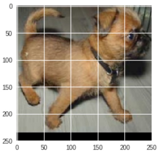
- Changed previous BGR to RGB using cv2 package. The images below show how the images looked before editing the images that were in the BGR format and after editing them to RGB.
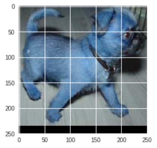 !
!
- Made y_test,y_train by putting their 10 classes to categorical.
We explored various neural network modifications for this dog breed classifcation project. Logistic Regression ——– A model with one flatten and one dense layer was evaluated to compare how our CNN’s and ResNets would compare to a simple logistical regresssion that would take in each image and output a classification result.
CNN
A CNN or Convolutional Neural Network is a type of deep learning that is commonly used for visual imagery analyzation , ideal for our dog breed classification project. This is because CNN add convolution layers that use learnable filters to find specific patterns or features from the original image. The filters are smaller but with the same number of dimensions for the image and same depth. For example, an image is usually read as a matrix of three dimensions, and the depth of three which takes into account the ‘color’ channels (rbg). If we have an image of size NXN the read matrix by the neural network has a matrix of size NXNX3. This would mean that a filter from a convolution layer is a matrix of size MXMX3 where M < N. Different filters detect different features in each image by sliding through all the spatial locations in the input image and creating a set of activation/feature maps as the output that goes into the next layer in the CNN.
Reference: He, K., Zhang, X., Ren, S. and Sun, J., 2016. Deep residual learning for image recognition. In Proceedings of the IEEE conference on computer vision and pattern recognition (pp. 770-778).
ResNet50
For this project we specifically looked at ResNET (Residual Neural Network) for our CNN model. ResNETs are a type of deep residual learning architecture commonly used for image recognition that facilitates the training of deeper networks. We used ResNET50 found Keras, the open-source neural network library. This ResNET follows the architechture by He et al. (2015) found here
VGG16
It is a pretrained imagenet model built using: Convolutions layers (used only 33 size ), Max pooling layers (used only 22 size), Fully connected layers at end. It has total of 19 layers. Below is a link about a mathworks implementation on vgg19 for more information. link on vgg19
Models and Performance
The table below shows the models used for this project and the results on the train and test sets. These were evaluated using model.evaluate(x,y).
| Model | Train Set Accuracy | Test Set Accuracy |
|---|---|---|
| Logistic Regression | 0.1615 | 0.1851 |
| CNN Baseline | 0.7093 | 0.1949 |
| CNN Edited Baseline version 1 | 0.3255 | 0.2375 |
| CNN Edited Baseline version 2 | 0.7093 | 0.2286 |
| CNN Edited Baseline version 3 | 0.5185 | 0.2537 |
| ResNET | 0.1615 | 0.1851 |
| VGG19 and Resnet | 0.948 | 0.2076 |
Logistic Regression
Epochs: 10, Learning Rate: 0.001, Batch Size: 24, Optimizer: SGD, Loss: categorical_crossentropy, validation split: 0.2, Parameters:1,875,010
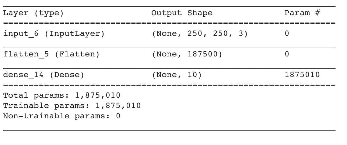 Our Logistic Regression Model performed as well as the ResNet Model but it was worse than our CNN models. It provides a good comparison on how much of the models below are over-complicated to the point where they do not improve the model performance.
Baseline Model (CNN)
Epochs: 15, Learning Rate: 0.1, Batch Size: 24, Optimizer: SGD, Loss: categorical_crossentropy, validation split: 0.2,parameters: 67,401,514
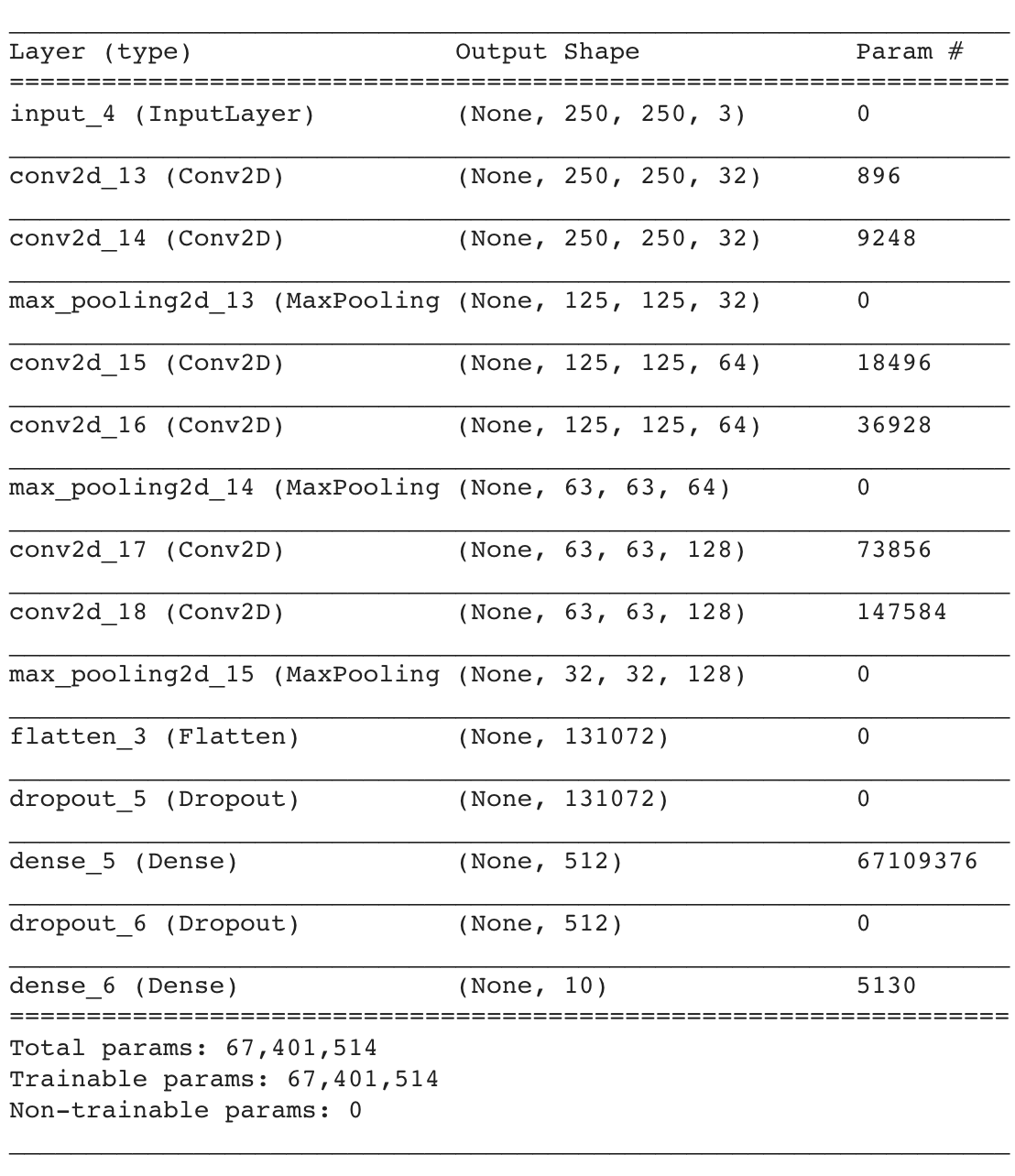 This model took ~40 minutes to fit. The loss did not converge, the epoch accuracies were also constant through the 15 epochs. This was later determined to be the coarse learning rate of 0.1 (Edited Baseline Model version 1). We later optimized the baseline model in in two different versions:
Edited Baseline Model version 1 (CNN)
Epochs: 15, Learning Rate: 0.01, Batch Size: 24, Optimizer: SGD, Loss: categorical_crossentropy, validation split: 0.2, parameters: 812,010
The Baseline CNN had over 67 million parameters , mostly exacerbated a 512 node dense overfitting layer that contributed to its 40 minute training time. Additionally its learning rate was 0.1, which may have lead to the non-decrease of the loss function. I decreased the learning rate to 0.01. I further reduced the parameters by increasing the number of max pooling layers, choosing to add one in between every one Conv2D layer instead of inbetween every two Conv2D layers.
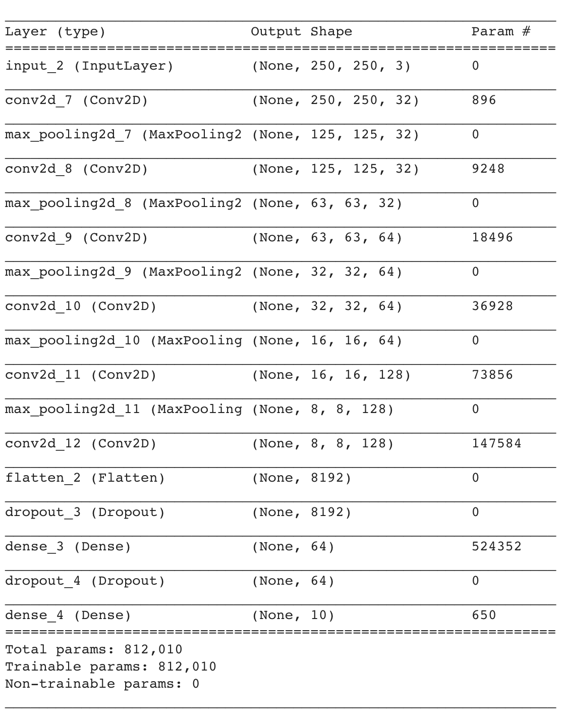
Compared to the baselin, the parameters are reduced to 812,000 and the training time is 15 minutes instead of 30. The overtraining is greatly reduced as well. The 2 drop-out layers(dropout_4 and dropout_3) each have 20% drop-out.
The training and validation accuracy versus epochs are shown in the figure below. The results show that as the number of epochs is increasing we have edited baseline cnn model decreasing in loss and increasing in accuracy with both training and test sets. The solid lines corresponds to the accuracy results on the left y-axis and the dotted lines correspond to the loss results on the right y-axis.
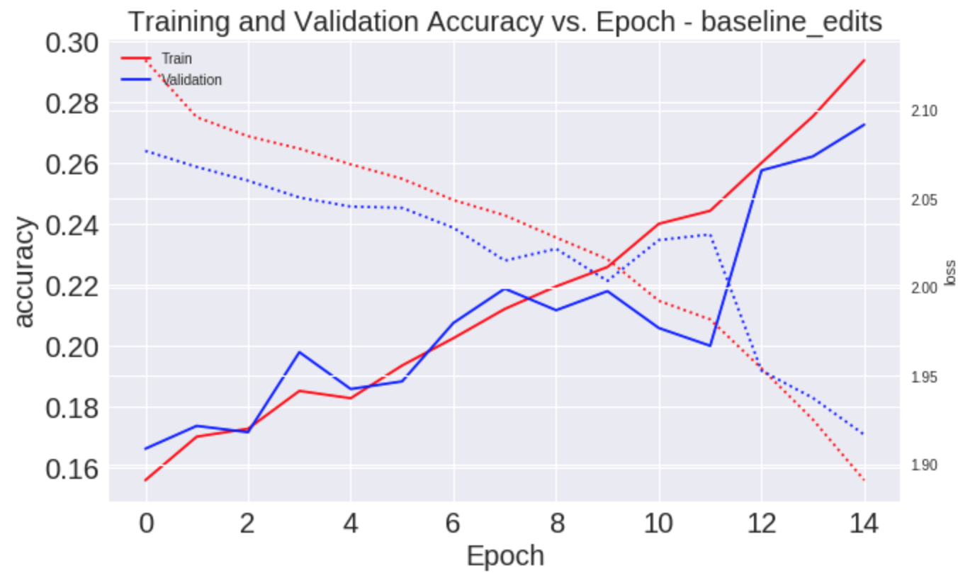
The loss and accuracy is not plateauing off so increasing the epochs would benefit this model. We wanted to show how fast the model could fit compared to the baseline so we kept the epochs at 15.
Edited Baseline Model version 2 (CNN)
Epochs: 10, Learning Rate: 0.01, Batch Size: 24, Optimizer: SGD, Loss: categorical_crossentropy, validation split: 0.2, parameters: 67,401,514
This model was not changed structurally from the baseline (summary for baseline is kept). It still has the 67 million+ parameters that leads to overfitting. The layers were kept the same as the baseline, but the learning rate was decreased from 0.1 to 0.01. The epochs were also decreased from 15 to 10 because it was overfitting after 10 epochs. It is apparent that the first edited version was much better and reduced overfitting than this version. The high contrast between train and test accuracy elucidates this.
Edited Baseline Model version 3 (CNN)
Epochs: 10, Learning Rate: 0.01, Batch Size: 24, Optimizer: SGD, Loss: categorical_crossentropy, validation split: 0.2, parameters: 812,010
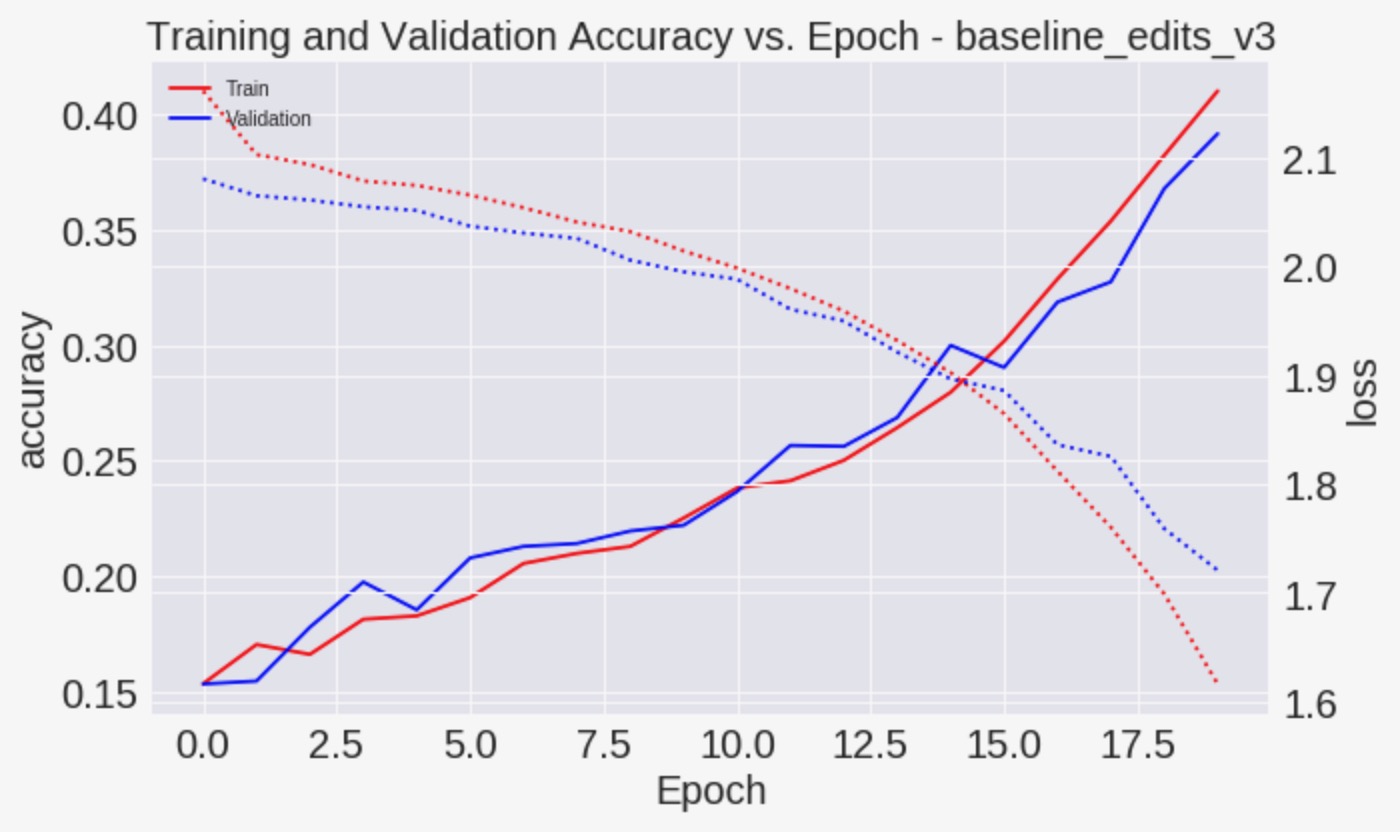
This model was not changed structurally from the baseline_edits_v1. The epochs were increased to 20 because it seemed like the previous baseline model v1 did not converge to a plateau. The final dropout before the final dense output layer is more aggressive at 30% dropout. The other dropout layer was kept the same. Judging from the plot of loss and accuracy, more epochs would possibly help the model fitting converge (similar to baseline model version 3). Other Learning Rates were experimented but they did not converge fast enough, additionally the loss for validation and train decreased monotonically implying that the learning rate was not too aggressive.
ResNet Model
Epochs: 8, Learning Rate: 0.000001, Batch Size: 24, Optimizer: Adam, Loss: categorical_crossentropy, validation split: 0.1, parameters: 23608202 non trainable, 20490 trainable
The ResNet model is pretrained on imagenet. The optional pooling mode for feature extraction applies global average pooling to the output of the last convolutional layer, meaning that the output would be a 2D tensor. We reduce the validation split to increase the training set. The learning rate is kept low to prevent the loss from jumping up and down, previous aggressive learning rates had non-monotonic loss.
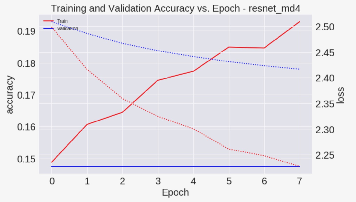
The validation does not show improvement. This can be due to poor fitting or small size of the validation set. The small validation set might have images difficult to be described by the model, no matter how trained the model might be. Data Augmentation will be able to improve the model, we would have to change our model fitting process to a fit generator which would flow the images in from the directory without using up RAM. Initial uses of ResNet had even higher overfitting tendencies and in this one, a dropout layer of 0.3 was added right before the final dense layer to prevent overfitting. Judging from the higher test accuracy than train accuracy, the biggest issue was not overfitting but rather could have been the insufficient number of training images or difficulty classifying into such diverse breed classifications.
VGGA16/ResNet combination
Epochs: 10, Batch Size: 4, Optimizer: rmsprop, Loss: categorical_crossentropy, validation split: 0.2, parameters: 1,532,682 non trainable, 2560 trainable
This model was implemented with 1000 images that were preprocessed differently: the x_train standardized by subtracting the channel mean and dividing by the standard deviation. Then we put the preprocessed input into pretrained models (Resnet and VGG19) and use model to extract features. The 2 outputs of these 2 model outputs were each put through a model that pooled the input, put it through a global average pooling layer, dense layer, normalize layer, and relu activation layer. Then the two tensor branches from each of the models were concatenated into one and fed into a dropout (0.3), dense (640), normalization, relu activation, dropout and dense layer.
The model structure is below
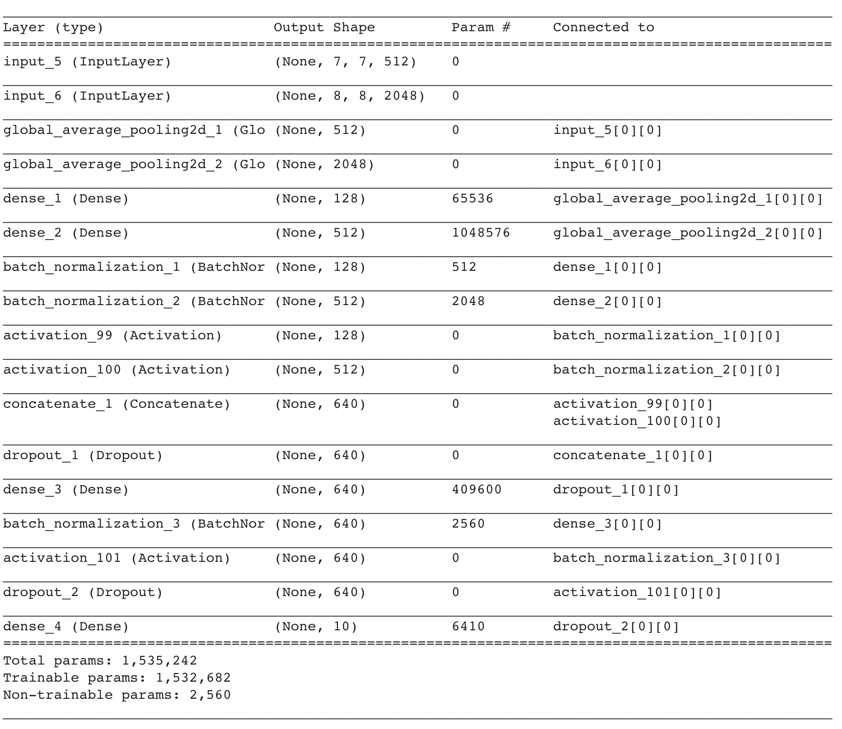 It is poor compared to the CNN model and does not improve significantly upon the logistic model. The code for this model is here: colab link to model. Better implementations would have more training data and perhaps more dropout layers to prevent overfitting. Less training data was used because the process for building the model and extracting the features generated too much RAM. Again, this process could be better tried with ImageDataGenerator flow_from_directory which would reduce the amount of RAM used.